Using fonts to format your worksheet
You can use different font, font size, font style, font color, and text attributes for your selection on the Font tab of the Format Cells dialog box (press Ctrl+1).
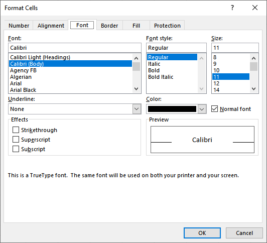
The screenshot below shows a few examples of font formatting.
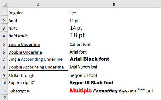
If a cell contains text (cannot work in values or formulas), you can use multiple formatting styles in a single cell:
If a cell contains text (as opposed to a value or a formula), you can apply formatting to individual characters in the cell. To do so,
- Switch to Edit mode (press F2, or double-click the cell)
- Select the characters that you want to format.
- Press Ctrl+1 to open the Format Cells dialog box and format the characters as you want.
By default, Excel uses the 11 point (pt) Calibri font, you can change it to suit your needs.
- Choose File > Options > General
- Under When creating new workbooks, select a font in the Use this as your default font field to change the default font, select a font size in the Font size field to change the default font size.
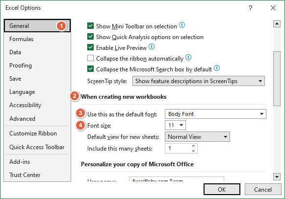
- Click Ok.
Changing text alignment
On the Alignment tab of the Format Cells dialog box (press Ctrl+1), you can see the full range of alignment options.

Horizontal alignment options
| General | Aligns numbers to the right, aligns text to the left, and centers logical and error values. This option is the default horizontal alignment. |
| Left | Aligns the cell contents to the left side of the cell. If the text is wider than the cell, the text spills over to the cell on the right. If the cell on the right isn't empty, the text is truncated and not completely visible. This is also available on the Ribbon. |
| Center | Centers the cell contents in the cell. If the text is wider than the cell, the text spills over to cells on either side if they're empty. If the adjacent cells aren't empty, the text is truncated and not completely visible. This is also available on the Ribbon. |
| Right | Aligns the cell contents to the right side of the cell. If the text is wider than the cell, the text spills over to the cell on the left. If the cell on the left isn't empty, the text is truncated and not completely visible. This is also available on the Ribbon. |
| Fill | Repeats the contents of the cell until the cell's width is filled. If cells to the right also are formatted with Fill alignment, they also are filled. |
| Justify | Justifies the text to the left and right of the cell. This option is applicable only if the cell is formatted as wrapped text and uses more than one line. |
| Center Across Selection | Centers the text over the selected columns. This option is useful for centering a heading over a number of columns. |
| Distributed | Distributes the text evenly across the selected column. |
If you choose Left, Right, or Distributed, you can also adjust the Indent setting, which adds horizontal space between the cell border and the text.
Vertical alignment options
| Top | Aligns the cell contents to the top of the cell. This is also available on the Ribbon. |
| Center | Centers the cell contents vertically in the cell. This is also available on the Ribbon. |
| Bottom | Aligns the cell contents to the bottom of the cell. This is also available on the Ribbon. This option is the default vertical alignment. |
| Justify | Justifies the text vertically in the cell; this option is applicable only if the cell is formatted as wrapped text and uses more than one line. This setting can be used to increase the line spacing. |
| Distributed | Distributes the text evenly vertically in the cell. |
Wrap Text and Shrink to Fit options
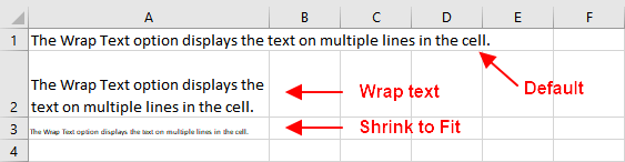
The Wrap Text option displays the text on multiple lines in the cell, if necessary. Use this option to display lengthy headings without having to make the columns too wide and without reducing the size of the text.
The Shrink to Fit option reduces the size of the text so that it fits into the cell without spilling over to the next cell. The times that this command is useful seem to be rare. Unless the text is just slightly too long, the result is almost always illegible.
The screenshot below shows the effect of "Wrap Text" and "Shrink to Fit".
If you apply Wrap Text formatting to a cell, you can't use the Shrink to Fit formatting.
Merge cells
You can use merge cells to create additional text space.
You can merge any number of cells occupying any number of rows and columns.
The range that you intend to merge should be empty, except for the upper-left cell. If any of the other cells that you intend to merge are not empty, Excel displays a warning. If you continue, all of the data (except in the upper-left cell) will be deleted.
You can use the Alignment tab of the Format Cells dialog box to merge cells, but using the Merge & Center control in the Alignment group on the Ribbon (or on the Mini toolbar) is simpler.
To merge cells, select the cells that you want to merge and then click the Home > Alignment > Merge & Center button. The Merge & Center button acts as a toggle.
To unmerge cells, select the merged cells and click the Merge & Center button again.
The Home > Alignment > Merge & Center control contains a drop-down list with these additional options:
- Merge Across: When a multirow range is selected, this command creates multiple merged cells—one for each row.
- Merge Cells: Merges the selected cells without applying the Center attribute.
- Unmerge Cells: Unmerges the selected cells.
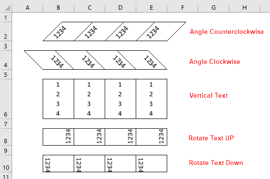
Orientation
You can display text horizontally, vertically, or at any angle between 90 degrees up and 90 degrees down.
From the Home > Alignment > Orientation drop-down list, you can apply the most common text angles.
For more control, use the Alignment tab of the Format Cells dialog box (press Ctrl+1). In the Format Cells dialog box, use the Degrees spinner control—or just drag the red pointer in the gauge. You can specify a text angle between –90 and +90 degrees.
The screenshot below shows the effect.
Right-to-Left
By default, text direction is set to Context, which means that text and numbers are aligned according to the language of the first character entered. For example, text in the cell is right-aligned if the first character is from a right-to-left language, and text is left-aligned if the first character in the cell is from a left-to-right language.
Using colors and shading
You control the color of the cell's text by choosing Home > Font > Font Color. Control the cell's background color by choosing Home > Font > Fill Color. Both of these color controls are also available on the Mini toolbar, which appears when you right-click a cell or range. Additional, you can also use the Fill tab of the Format Cells dialog box to apply different styles and colors to your cells.
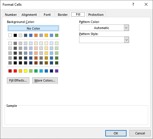
Background Color
Pick the color you want to use as the background color for the selected cell from the provided color options.
Click the No Color button to remove any color from the selected cell.
Click the Fill Effects button to open the Fill Effects dialog box. From there you can select different gradients and shading styles.
Click the More Colors button to open the Colors dialog box. From there you can choose from more color options or create a custom color to use for your formatting.
To hide the contents of a cell, make the background color the same as the font text color. The cell contents are still visible in the Formula bar when you select the cell. Keep in mind, however, that some printers may override this setting, and the text may be visible when printed.
Pattern Color
To use a pattern with two colors, click another color in the Pattern Color box, and then click a pattern style in the Pattern Style box.
If you choose a gradient or shading effect through the Fill Effects button, Excel sets the Pattern Color box to Automatic.
Pattern Style
Select a pattern style to use for your cell formatting. Excel provides various options for dots, stripes, and lines here. The default option is no pattern style.
Sample
In the Sample box, you can preview the background, pattern, and fill effects you selected.
Apply or remove cell borders
You can quickly apply or remove cell borders in the Home > Font > Borders drop-down list.
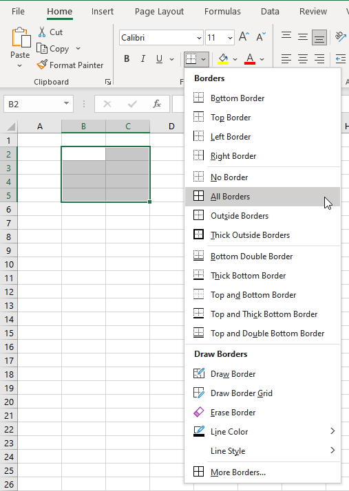
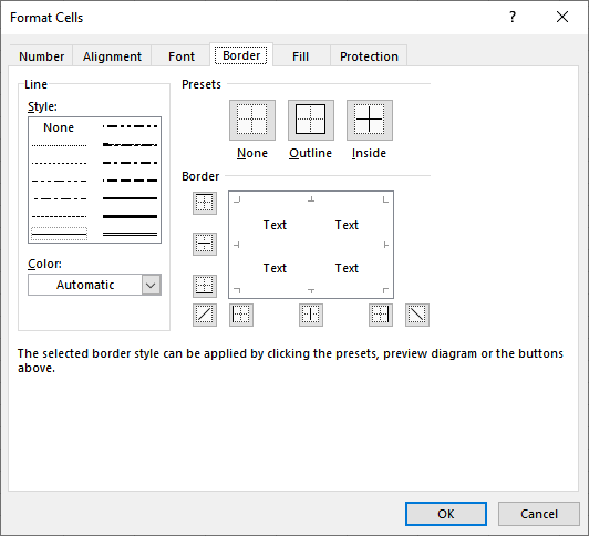
You can use the Border tab of the Format Cells dialog box for more control over cell borders.
If you use border formatting in your worksheet, you may want to turn off the grid display to make the borders more pronounced. Choose View > Show > Gridlines to toggle the gridline display.
Copying Formats by Format Painte
The quick and easy way to copy the formats from one cell to another cell or range is to use the Format Painter button of the Home > Clipboard group.
- Select the cell or range that has the formatting attributes that you want to copy.
- Click the Format Painter button. The mouse pointer changes to include a paintbrush.
- Select the cells to which you want to apply the formats.
- Release the mouse button, and Excel applies the same set of formatting options that were in the original range.
- If you double-click the Format Painter button, you can paint multiple areas of the worksheet with the same formats. Excel applies the formats that you copy to each cell or range that you select. To get out of Paint mode, click the Format Painter button again (or press Esc).