Using Tables in Formulas

Create an Excel table

1. Click any cell in a data list.
2. Go to the Styles group on the Home tab.
3. Click Format as Table.
4. In the gallery that appears, click the style you want to apply.
5. In the Format As Table dialog box, verify that Excel has identified the correct cell range, check the My table has headers box if appropriate, and click OK.

Using structured references with Excel tables

When you create an Excel table, Excel assigns a name to the table and to each column header in the table. When you add formulas to an Excel table, these names are automatically displayed when you enter formulas and select cell references in the table, rather than having to enter them manually. For example:

using explicit cell references	using table and column names
=Sum(C2:C9)	=SUM(Table1[Sales Amount])

That combination of table and column names is called a structured reference. The names in structured references adjust whenever you add or remove data from the table.

Structured references also appear when you create a formula outside of an Excel table that references table data. The references can make it easier to locate tables in a large workbook.

To include structured references in your formula, click the table cells you want to reference instead of typing their cell reference in the formula.

Example

Let’s use the following example data to enter a formula that automatically uses structured references to calculate the amount of a sales commission.

Sales Person	Region	Sales Amount	Commission Rate	Commission Amount
Nancy	North	480	12%
Andy	South	720	14%
Jan	East	840	13%
Mariya	West	520	12%
Steven	North	780	11%
Michael	South	870	12%
Robert	East	900	15%
Bob	West	680	12%

1. Copy the sample data in the table above, including the column headings, and paste it into cell A1 of a new Excel worksheet.
2. Select any cell within the data range, and press Ctrl+T.
3. Make sure the My table has headers box is checked, and click OK.
4. A table named Table1 is created (the default name for the first table you create in a workbook).
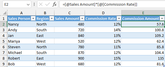
5. In cell E2, type an equal sign (=), and click cell C2.
6. In the formula bar, the structured reference [@Sales Amount] appears after the equal sign.
7. Type an asterisk (*) directly after the closing bracket, and click cell D2.
8. In the formula bar, the structured reference [@[Commission Rate]] appears after the asterisk.
9. Press Enter.
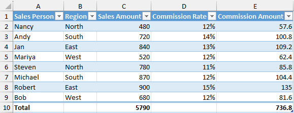
10. Excel automatically creates a calculated column and copies the formula down the entire column for you, adjusting it for each row.

Change a table name

When you create an Excel table, Excel creates a default table name (Table1, Table2, and so on), but you can change the table name to make it more meaningful.

1. Select any cell in the table to show the Table Design tab on the ribbon.
2. Type the name you want in the Table Name box, and press Enter.

In our example data, we used the name RegionSales.

Rules for table names

• Use valid characters: Always start a name with a letter, an underscore character (_), or a backslash (\). Use letters, numbers, periods, and underscore characters for the rest of the name. You can’t use "C", "c", "R", or "r" for the name, because they’re already designated as a shortcut for selecting the column or row for the active cell when you enter them in the Name or Go To box.
• Don’t use cell references: Names can’t be the same as a cell reference, such as A$100 or R1C1.
• Don’t use a space to separate words: Spaces can’t be used in the name. You can use the underscore character (_) and period (.) as word separators. For example, RegionSales, Income_Tax or Second.Quarter.
• Use no more than 255 characters: A table name can have up to 255 characters.
• Use unique table names: Duplicate names aren’t allowed. Excel doesn’t distinguish between upper and lowercase characters in names so if you enter “Sales” but already have another name called “SALES" in the same workbook, you’ll be prompted to choose a unique name.
• Use an object identifier: If you plan on having a mix of tables, PivotTables and charts, it's a good idea to prefix your names with the object type. For example: tbl_Sales for a sales table, pt_Sales for a sales PivotTable, and chrt_Sales for a sales chart, or ptchrt_Sales for a sales PivotChart. This keeps all of your names in an ordered list in the Name Manager.

Structured reference syntax rules

Basic Structure

TableName[[Item Specifier],[Column Specifier1]:[Column Specifier2]]

Components

1. TableName: This refers to the assigned name of your Excel table.
2. Item Specifier: This can only be one of the following:
   • #All: The entire table, including column headers, data, and totals (if any).
   • #Data: Refers to all rows containing data (excluding headers and totals).
   • #Headers: Refers to all rows containing table headers.
   • #Totals: Just the total row. If none exists, then it returns null.
   • #This Row or @ or @[Column Name]: Just the cells in the same row as the formula. Excel automatically changes #This Row specifiers to the shorter @ specifier in tables that have more than one row of data.
3. Column Specifier: This identifies the column(s) you want to reference. You can use:
   • Column Header: directly using the header name without brackets (e.g., Sales Amount).
   • ColumnRange: specifying a range of columns using colons (e.g., [Sales Amount]:[Commission Amount]).

Let’s look at the following formula example to help understand structured reference syntax:

=SUMIF(RegionSales[Region],"North",RegionSales[Commission Amount])/RegionSales[[#Totals],[Commission Amount]]

This formula has the following structured reference components:

• Table name: RegionSales is a custom table name. It references the table data, without any header or total rows. You can use a default table name, such as Table1, or change it to use a custom name.
• Column specifier: [Region] and [Commission Amount] are column specifiers that use the names of the columns they represent. They reference the column data, without any column header or total row. Always enclose specifiers in brackets as shown.
• Item specifier: [#Totals] is special item specifiers that refer to specific portions of the table, such as the total row.
• Table specifier: [[#Totals],[Commission Amount] is table specifiers that represent the outer portions of the structured reference. Outer references follow the table name, and you enclose them in square brackets.
• Structured reference: RegionSales[Region], RegionSales[Commission Amount] and RegionSales[[#Totals],[Commission Amount]] are structured references, represented by a string that begins with the table name and ends with the column specifier.

Remarks

Use an escape character for some special characters in column headers

Some characters have special meaning and require the use of a single quotation mark (') as an escape character. Here’s the list of special characters in the formula:

• Left bracket ([)
• Right bracket (])
• Pound sign(#)
• Single quotation mark (')
• At sign (@)

For example: =RegionSales['#Items].

Use the space character to improve readability in a structured reference

It’s recommended to use one space:

• After the first left bracket ([).
• Preceding the last right bracket (]).
• After a comma (,).

For example: =RegionSales[ [#Headers], [#Data], [Sales Amount]:[Commission Amount] ]

Use the reference operators to combine column specifiers

• : (colon) range operator
• , (comma) union operator
• (space) intersection operator

Qualifying structured references in calculated columns

If you’re using structured references within a table, such as when you create a calculated column, you can use an unqualified structured reference, but if you use the structured reference outside of the table, you need to use a fully qualified structured reference.

For example:

Unqualified: =[@[Sales Amount]]*[@[Commission Rate]]

Fully qualified: =RegionSales[@[Commission Rate]]*RegionSales[@[Commission Amount]]

Examples

The following structured reference example is based on the previous data.

Structured reference	Cell range
=RegionSales[[#All],[Sales Amount]]	C1:C10
=RegionSales[[#All],[Sales Amount]:[Commission Amount]]	C1:E10
=RegionSales[[#Totals],[Sales Amount]]	C10
=RegionSales[[#Totals],[Sales Amount]:[Commission Amount]]	C10:E10
=RegionSales[[#Headers],[Commission Amount]]	E1
=RegionSales[[#Headers],[Region]:[Commission Amount]]	B1:E1
=RegionSales[[#Headers],[#Data],[Commission Amount]]	E1:E9
=RegionSales[[Commission Rate]:[Commission Amount]]	D2:E9
=RegionSales[@[Commission Amount]]	E9 (if the current row is 9)