Description
T function returns the text referred to by value.
Syntax
T(value)Parameters
value Required. The value you want to test.
Remarks
- If value is or refers to text, T returns value. If value does not refer to text, T returns "" (empty text).
- You do not generally need to use the T function in a formula because Microsoft Excel automatically converts values as necessary. This function is provided for compatibility with other spreadsheet programs.
Examples
Example 1: check for valid numbers
The example may be easier to understand if you copy the example data (include header) in the following table, and paste it in cell A1 of a new Excel worksheet. If you need to, you can adjust the column widths to see all the data.
| Data | Formula | Result | Description |
|---|---|---|---|
| Excel | =T(A2) |
Excel | Because the value is text, the text is returned. |
| 12/24/2014 | =T(A3) |
Because the value is a data value, empty text is returned. | |
| 15:04 | =T(A4) |
Because the value is a time value, empty text is returned. | |
| TRUE | =T(A5) |
Because the value is a logical value, empty text is returned. | |
| FALSE | =T(A6) |
Because the value is a logical value, empty text is returned. | |
| 2013 | =T(A7) |
Because the value is a number, empty text is returned. |
Example 2: list worksheet names
- On the Formulas tab, in the Defined Names group, click Define Name.
- In the New Name dialog box, in the Name box, type the name that you want to use for your reference, for this example, type
SheetName. - To specify the scope of the name, in the Scope drop-down list box, select Workbook or the name of a worksheet in the workbook. In this example, we select Workbook.
- Optionally, in the Comment box, enter a descriptive comment up to 255 characters, in this example we type:
Get worksheet names - In the Refers to box, enter the formula:
=GET.WORKBOOK(1)&T(NOW())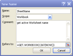
- To finish and return to the worksheet, click OK.
- Use the defined Name: in cell A1 or wherever you want the worksheet name to appear, enter the formula:
=REPLACE(INDEX(SheetName,ROW(A1)),1,FIND("]",INDEX(SheetName,ROW(A1))),)or:
=MID(INDEX(SheetName,ROW(A1)),FIND("]",INDEX(SheetName,ROW(A1)))+1,255)Now, you will get the first worksheet name. Dragging down the formula to get all worksheet names.
If you change any worksheet Name, A1 will automatic change the value immediately.
If you want to create a hyperlink to the worksheet, use the following formula:
=HYPERLINK(INDEX(SheetName,ROW(A1))&"!A1",REPLACE(INDEX(SheetName,ROW(A1)),1,FIND("]",INDEX(SheetName,ROW(A1))),))or
=HYPERLINK(INDEX(SheetName,ROW(A1))&"!A1",MID(INDEX(SheetName,ROW(A1)),FIND("]",INDEX(SheetName,ROW(A1)))+1,255))Why don't we define the SheetName as =INDEX(GET.WORKBOOK(1)&T(NOW()),ROW(A1))?
If you do, select cell "A1" in step 1, and define the SheetName.
The formula only working begin with Row 1, eg. A1, B1, C1...
Why use T(NOW()) formula? Because use T(NOW()) formula you don't need to recalculate the formula, it'll return the value immediately.
Furthermore, you can use CELL function To get active Worksheet name.