Using Names in Excel Formulas

For basic information on using names, see Working with Range Names.

Applying names to existing references

When you create a name for a cell or a range, Excel doesn't automatically replace the existing references with the name in the formulas.

For example, suppose you have the following formula in cell H13:

=SUM(H2:H12)

If you later define a name TotalPrice for H2:H12, Excel won't automatically change your formula to =SUM(TotalPrice).

To replace range references with their names in formulas:

1. Select the range that you want to replace. If you select only one cell, the entire active worksheet will be replaced.
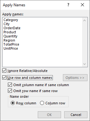
2. Choose Formulas > Defined Names > Define Name > Apply Names to open Apply Names dialog box (or press Alt+MMA).
   
3. (Optional) You can click the Options button to expand the Apply Names dialog box.
   • Ignore Relative/Absolute: Most of the time, you’ll want to leave this check box selected because Excel automatically assigns absolute cell references to the names that you define and relative cell references to the formulas that you build. If you want Excel to replace only those cell references that use the same type of references as are used in your names (absolute for absolute, mixed for mixed, and relative for relative), deselect this check box.
   • Use Row and Column Names: The names created from row and column headings with the Create Names command appear in your formulas. Deselect this option if you don’t want these row and column names to appear in the formulas in your worksheet.
   • Omit Column Name If Same Column: This prevents Excel from repeating the column name when the formula is in the same column. Deselect this check box when you want the program to display the column name even in formulas in the same column as the heading used to create the column name.
   • Omit Row Name If Same Row: This prevents Excel from repeating the row name when the formula is in the same row. Deselect this check box when you want the program to display the row name even in formulas in the same row as the heading used to create the row name.
   • Name Order: Click the Row Column option button (the default) if you want the row name to precede the column name when both names are displayed in the formulas, or click the Column Row option button if you want the column name to precede the row name.
4. Select the names you want to apply by clicking them.
5. Click OK.
6. Excel replaces the range references with the names in the selected range.

Using names for constants

In addition to naming cells in a worksheet, you can also assign names to constants that doesn't appear in a cell.

For example, if the formula in the worksheet uses a discount rate, you might insert the value of the discount rate into a cell and use a reference to this cell in the formula. For convenience, you might also name this cell something like DiscountTax. You can also provide a name for a value that does not appear in the cell.

Here's how to assign a constant value of 10% to the range name DiscountRate:

1. Choose Formulas > Defined Names > Define Name. Excel opens the New Name dialog box (or press Alt+MMD).
2. Enter the name (in this case, DiscountTax) into the Name field.
   
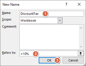
3. (Optional) Select a scope in which the name will be valid (either the entire workbook or a specific worksheet).
4. In the Refers To text box, enter a new value (=10%).
5. (Optional) Use the Comment box to provide a comment about the name.
6. Click OK.

You just created a name that refers to a constant rather than a cell or range. Now if you type =DiscountTax into a cell that's within the scope of the name, this simple formula returns 0.1 (the constant that you defined). You can also use this constant in a formula, such as =A2*DiscountTax.

Using names for formulas

In addition to creating named constants, you can create named formulas. For example, you can create a named formula to calculate an arithmetic expression. In this example, range A2:A8 contains arithmetic expressions, range B2:B8 is the result, the name Calc refers to the following formula:

=EVALUATE(Sheet1!A2)

Note that the EVALUATE function is a macro function and cannot be used directly in an Excel worksheet, you need to create a name to use it.

1. Activate worksheet Sheet1 and select cell B2, and assign the formula =EVALUATE(Sheet1!A2) to the range name Calc:
   1. Choose Formulas > Defined Names > Define Name. Excel opens the New Name dialog box (or press Alt+MMD).
   2. In the Name field, type Calc.
      
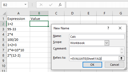
   3. (Optional) Select a scope in which the name will be valid (either the entire workbook or a specific worksheet).
   4. In the Refers To text box, type =EVALUATE(Sheet1!A2).
   5. (Optional) Use the Comment box to provide a comment about the name.
   6. Click OK.
2. In cell B2, enter the formula =Calc and press Enter.
3. Drag the Fill handle in cell B2 down to cell B8 and release the mouse button to copy the formula.
4. The result:
   

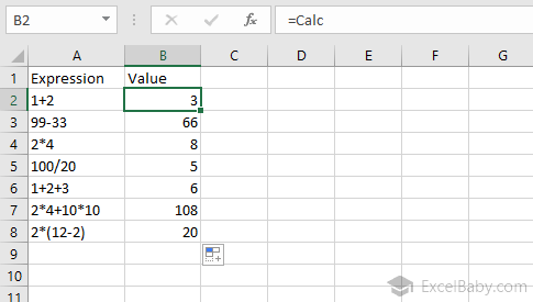
Note that in this example, the formula =EVALUATE(Sheet1!A2) is a relative reference.

When you use the pointing technique to create a formula in the Refers To field of the New Name dialog box, Excel always uses absolute cell references, you can press F4 several times to convert the current cell reference to relative or type in the cell address without dollar signs.

Using range intersections

Intersection operator

Excel uses a space character to identify overlapping references in two ranges, and the space between the row and column names is called the intersection operator.

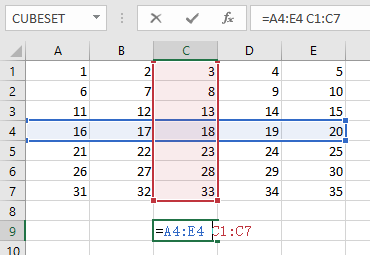
The following figure shows a simple example.

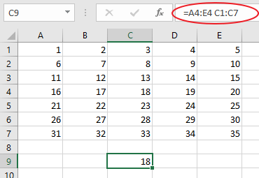
The formula in cell C9 is =A4:E4 C1:C7, this formula returns 18, the value in cell C4, that is, the value at the intersection of the two ranges. If you double-click on cell C4, you will see that the range A4:E4 intersects with the range C1:C7 at cell C4.

The following table shows the reference operators in Excel, in Excel 365 or later, you will see the spilled range operator (#) and the implicit intersection operator (@). For more informations, see: Use Calculation Operators in Excel Formulas.

Reference operator	Meaning	Example
: (colon)	Range operator, which produces one reference to all the cells between two references, including the two references.	=A1:A15
, (comma)	Union operator, which combines multiple references into one reference	=SUM(A1:A15,D1:D15)
(space)	Intersection operator, which produces one reference to cells common to the two references	=A4:D4 C1:C8

Example of range intersections

The following table shows the number of sales per quarter for each of the four cities.

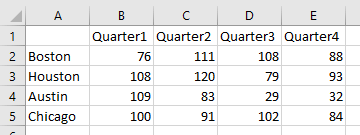
We selected the range A1:E5 and then chose Formulas > Defined Names > Create from Selection to create names automatically by using the top row and the left column.

Excel created the following eight names:

Austin	=Sheet1!$B$4:$E$4
Boston	=Sheet1!$B$2:$E$2
Chicago	=Sheet1!$B$5:$E$5
Houston	=Sheet1!$B$3:$E$3
Quarter1	=Sheet1!$B$2:$B$5
Quarter2	=Sheet1!$C$2:$C$5
Quarter3	=Sheet1!$D$2:$D$5
Quarter4	=Sheet1!$E$2:$E$5

Naming ranges in this way can help you create very readable formulas.

To calculate the total for Quarter1, just use this formula:

=SUM(Quarter1)

To refer to a single cell, use the intersection operator, just use this formula:

=Chicago Quarter3

This formula returns the value for the third quarter for the Chicago city. In other words, it returns the value that exists where the Quarter3 range intersects with the Chicago range.