Creating Formulas

Create a formula

1. Select a cell.
2. Type an equal sign (=).
   Note: The first character in a cell containing a formula must be =. If it is any other character, including a space, Excel interprets the cell’s contents as text.
3. Select a cell or type its address in the selected cell.
   

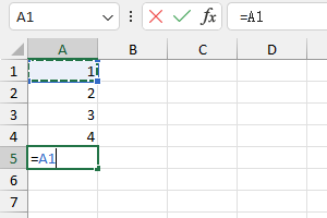
   Select a cell

4. Enter an operator. For example, + for addition.
5. Select the next cell, or type its address in the selected cell.
   

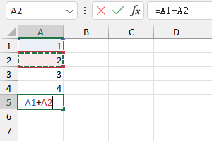
   Select the next cell

6. Press Enter. The result of the operation will be displayed.

Refer to cells & cell ranges in formulas

• Worksheet cells are identified by their column letter and then their row number.
• The top-left cell in a worksheet is in column A and row 1, so its cell address is A1.
• You can also refer to cell ranges, or collections of cells.
• To identify a cell range, type the address of the cell at the topleft corner of the range, followed by a colon (:), and then the cell at the bottom-right corner of the range. For Example, the reference for cells 1 through 5 in columns A and B would be A1:B5.
• To create a reference to multiple, noncontiguous groups of cells, put a comma (,) between the references. For Example, finding the sum of the values in the cell range A2:B6 and the range D2:E6 would call for the formula =SUM(A2:B6,D2:E6).

Create relative, absolute & mixed references

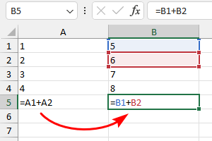
Relative reference

When you type a cell reference with just the column letter and row number, such as A1, that reference can change when you copy its formula to another cell.

For Example, copying the formula =A1+A2 and pasting it one cell to the right would create the formula =B1+B2. The destination cell is one column to the right of the original cell, so Excel changes the formula’s references based on that difference.

Relative reference

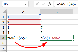
Absolute reference

To create an absolute reference, one that doesn’t change when you copy a formula, type a dollar sign ($) before the column and row designators.

For Example, the formula =$A$1+$A$2 won’t change regardless of the cell you paste it into.

Absolute reference

Mixed reference

You can also create a mixed reference, where either rows or columns are absolute, by adding $ before just the element you want to remain the same.

For Example, the cell reference A$1 allows changing columns and $A1 allows changing rows.

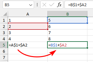
Mixed reference

Switch the types of your references

1. Select the cell that contains the formula.
2. In the formula bar, select the reference that you want to change.
3. Press F4 to switch between the reference types.
   

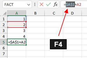
   Press F4 to switch between the reference types

Reference cells outside the worksheet

Formulas can also refer to cells in other worksheets, and the worksheets don't even have to be in the same workbook. Excel uses a special type of notation to handle these types of references.

Reference cells in other worksheets

To use a reference to a cell in another worksheet in the same workbook, use this format:

=SheetName!CellAddress

In other words, precede the cell address with the worksheet name followed by an exclamation point. For example:

=A1-Sheet2!A1

=B2*'Sales Dept'!$A$2

Reference cells in other workbooks

To refer to a cell in a different workbook, use this format:

=[WorkbookName]SheetName!CellAddress

In this case, the workbook name (in square brackets), the worksheet name, and an exclamation point precede the cell address. For example:

=[Sales.xlsx]Sheet1!A1

If the workbook name in the reference includes one or more spaces, you must enclose it (and the sheet name and square brackets) in single quotation marks. For example:

=A1*'[Sales For 2023.xlsx]Sheet1'!A1

When a formula refers to cells in a different workbook, the other workbook doesn't have to be open. If the workbook is closed, however, you must add the complete path to the reference so that Excel can find it. For example:

=A1*'C:\My Documents\[Sales For 2023.xlsx]Sheet1'!A1

A linked file can also reside on another system that's accessible on your corporate network. The following formula refers to a cell in a workbook in the files directory of a computer named MyDataServer:

='\\MyDataServer\files\[Sales For 2023.xlsx]Sheet1'!A1

or IP address:

='\\192.168.0.2\files\[Sales For 2023.xlsx]Sheet1'!A1

Insert a function

Start creating the formula where you want to insert the function, and then do one of the following:

• Type the first letters of the function name, and either finish typing its name, or click the function on the AutoComplete list that appears and press Tab. For example, =SUM for getting the total numbers:
  1. Click the cell A5 and type =s.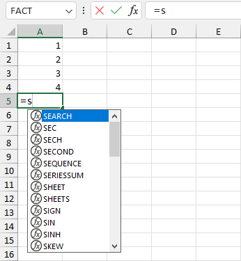
     

     Type the first letters of the function name

  2. Excel lists functions that match so far, so you can select a function and see its description, scroll down to see more names, or continue typing. For example, =su to narrow the list.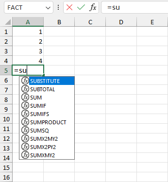
     

     Type su to narrow the list

  3. When you find the function that you require, double-click the name or press Tab, then enter the arguments that are shown. For example, double-click SUM, then click range A1:A4.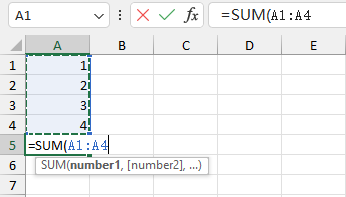
     

     Enter the arguments

  4. Type the closing parenthesis ()), and then press Enter.
  5. The formula with the function is stored in the cell =SUM(A1:A4), and the result of the operation will be displayed.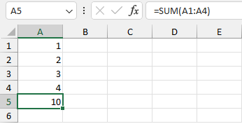
     

     Display operation results

• Click the Insert Function button on the Formulas tab and select the function you want to add. Or use shortcut: Shift+F3
  

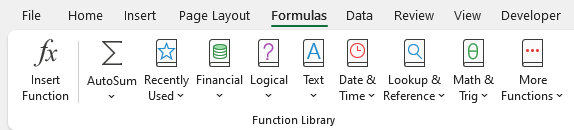
  Insert Function

• Go to the Function Library group on the Formulas tab, click the category of the function you want to add, and then click the function name.

Add an AutoSum function

1. Select a cell below a column of numbers.
2. Go to the Editing group on the Home tab.
3. Click the AutoSum button to add a SUM formula, or click the AutoSum button’s down arrow to select another function.

Get help using function argument ToolTips

• Start creating a formula, and enter the name of the function followed by a left parenthesis, such as =SUMIF(.
• In the function ToolTip that appears below the cell that contains the formula, position the mouse pointer over the function name.
• When the function name’s text changes to a blue, underlined format, click it to display the function help.
  

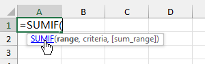
  Get function help