Evaluate Formula

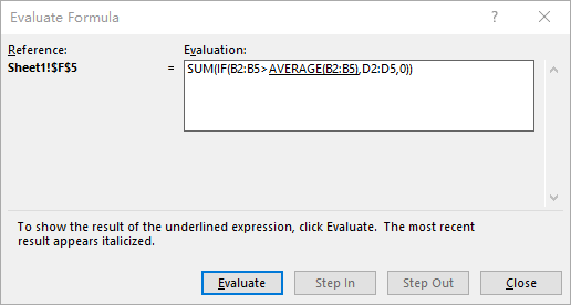
Sometimes, understanding nested formulas can be difficult, especially long and complex formulas! However, by using the Evaluate Formula dialog box, you can break down the formula calculation sequence step by step so that you can understand it.

Let's see how to solve the formula =SUM(IF(B2:B5>AVERAGE(B2:B5),D2:D5,0)) with the following example:

Evaluate formulas example

1. Select the cell that you want to evaluate. Only one cell can be evaluated at a time. In this example, we select cell F5.
2. On the Formulas tab, in the Formula Auditing group, click Evaluate Formula.
   

   Evaluate Formulas Ribbon

3. Click Evaluate to examine the value of the underlined reference. The result of the evaluation is shown in italics.
   

   Evaluate Formula dialog box

4. If the underlined part of the formula is a reference to another formula, click Step In to display the other formula in the Evaluation box. Click Step Out to go back to the previous cell and formula.
   Note: The Step In button is not available for a reference the second time the reference appears in the formula, or if the formula refers to a cell in a separate workbook.
5. Continue until each part of the formula has been evaluated.
6. To see the evaluation again, click Restart.
7. To end the evaluation, click Close.
8. The detailed evaluate steps of the formula are listed below:
   1. =SUM(IF(B2:B5>AVERAGE(B2:B5),D2:D5,0))
   2. =SUM(IF({450;550;720;850}>642.5,D2:D5,0))
   3. =SUM(IF({FALSE;FALSE;TRUE;TRUE},D2:D5,0))
   4. =SUM({0;0;108;102})
   5. =210