Description
REPT function repeats a piece of text a specified number of times. Use REPT to fill a cell with a number of instances of a text string.
Syntax
REPT(text,number_times)Parameters
text: is the character or string you want to repeat
number_times: is the number of times to repeat text
Remarks
- If number_times is 0 (zero), REPT returns "" (empty text).
- If number_times is omitted, REPT returns "" (empty text).
- If number_times is not an integer, it is truncated.
- The result of the REPT function cannot be longer than 32,767 characters, or REPT returns #VALUE!.
The example may be easier to understand if you copy the example data (include header) in the following table, and paste it in cell A1 of a new Excel worksheet. If you need to, you can adjust the column widths to see all the data.
| Formula | Result | Description |
|---|---|---|
=REPT("A",0) |
number_times is 0 (zero), REPT returns "" (empty text). | |
=REPT("A",) |
number_times is omitted, REPT returns "" (empty text). | |
=REPT("A",32768) |
#VALUE! | number_times > 32767, returns #VALUE! |
=REPT("A",3.9) |
AAA | number_times is not an integer, it is truncated, 3.9=3. |
Examples
Padding a Cell
The REPT function is sometimes used to pad a cell with characters.
The example may be easier to understand if you copy the example data (include header) in the following table, and paste it in cell A1 of a new Excel worksheet. If you need to, you can adjust the column widths to see all the data.
| Formula | Result | Description |
|---|---|---|
=REPT("-",5) |
----- | displays a dash 5 times. |
=REPT(".",3)&" by Excelbaby.com" |
... by Excelbaby.com | add leading dots in a cell. |
="Read More"&REPT(".",3) |
Read More... | add trailing dots in a cell. |
="<!-- "&REPT("*",6)&" -->" |
<!-- ****** --> | displays the string 6 times. |
Building Text Charts
A more common use for the REPT function is to build text-based charts.
In this case, you use a numeric result in a cell as the REPT function’s number argument, and the repeated character then charts the result.
You can format the chart cells with the Webdings font or Playbill font. if the character you want to repeat is g, please use Webdings font, if the character you want to repeat is |, please use Playbill font. see example:
The example may be easier to understand if you copy the example data (include header) in the following table, and paste it in cell A1 of a new Excel worksheet. If you need to, you can adjust the column widths to see all the data.
| Formula | Result | Description |
|---|---|---|
=REPT("g", 3) |
ggg | You need to change B2 font with Webdings |
=REPT("g", 3) |
ggg | B3 font: Calibri |
=REPT("|", 10) |
|||||||||| | You need to change B4 font with Playbill |
=REPT("|", 10) |
|||||||||| | B5 font: Calibri |
Result:

Column Sparkline
You can use the REPT function to create Column Sparkline.

1. Select A2:C2, and input below formulas:
=INT(RAND()*100)press Ctrl+Enter to end input.
2. Select D2, and input below formulas:
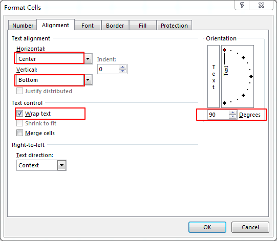
=REPT("|",A2/MAX($A2:$C2)*15)&CHAR(10)&REPT("|",B2/MAX($A2:$C2)*15)&CHAR(10)&REPT("|",C2/MAX($A2:$C2)*15)3. Select D2, press Ctrl+1, click Alignment, set:
Horizontal: Center
Vertical: Bottom
Choose Wrap text
Orientation = 90 Degrees

4. Set D2 font to Playbill and font color to blue.
5. If you need to, you can adjust the column heights and widths.
What's *15 mean in the formula REPT("|",A2/MAX($A2:$C2)*15)&CHAR(10)? The 15 is the height of sparkline, which can be set a little smaller than the row height, if the row height is 20 pixels, the formula can be set to 15, this means that the sparkline can be displayed completely on a row.
Data Bar
The example may be easier to understand if you copy the example data (include header) in the following table, and paste it in cell A1 of a new Excel worksheet. If you need to, you can adjust the column widths to see all the data.
| Data | Built-in Data Bar | Formula Data Bar | Description |
|---|---|---|---|
| =RAND()*1000 | =A2/MAX($A$2:$A$10) | =REPT("|",100*A2/MAX($A$2:$A$10)) | Set C2:C10 font with Playbill |
| =RAND()*1000 | =A3/MAX($A$2:$A$10) | =REPT("|",100*A3/MAX($A$2:$A$10)) | Set C2:C10 font with Playbill |
| =RAND()*1000 | =A4/MAX($A$2:$A$10) | =REPT("|",100*A4/MAX($A$2:$A$10)) | Set C2:C10 font with Playbill |
| =RAND()*1000 | =A5/MAX($A$2:$A$10) | =REPT("|",100*A5/MAX($A$2:$A$10)) | Set C2:C10 font with Playbill |
| =RAND()*1000 | =A6/MAX($A$2:$A$10) | =REPT("|",100*A6/MAX($A$2:$A$10)) | Set C2:C10 font with Playbill |
| =RAND()*1000 | =A7/MAX($A$2:$A$10) | =REPT("|",100*A7/MAX($A$2:$A$10)) | Set C2:C10 font with Playbill |
| =RAND()*1000 | =A8/MAX($A$2:$A$10) | =REPT("|",100*A8/MAX($A$2:$A$10)) | Set C2:C10 font with Playbill |
| =RAND()*1000 | =A9/MAX($A$2:$A$10) | =REPT("|",100*A9/MAX($A$2:$A$10)) | Set C2:C10 font with Playbill |
| =RAND()*1000 | =A10/MAX($A$2:$A$10) | =REPT("|",100*A10/MAX($A$2:$A$10)) | Set C2:C10 font with Playbill |
Result:

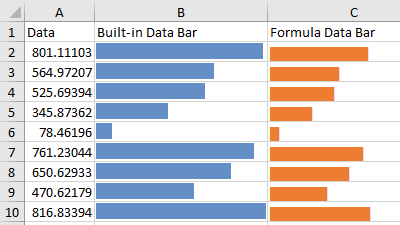
This example use REPT function to build Data Bar, you need to set C2:C10 font with Playbill. the formula data bar is almost the same as the Excel built-in data bar.
Excel built-in data bar:
- Select Range B2:B10
- Home > Styles > Conditional Formatting > Data Bars > Solid Fill > Blue Data Bar
- Hide the number of built-in data bar: Press CTRL + 1 and set the Number format with custom code:
;;;