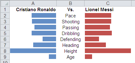
Tornado Chart is a special type of Bar Chart, also called Tornado Diagram. Tornado Chart is useful for deterministic sensitivity analysis. We usually building Tornado Chart with Bar Chart, but in this tutorial, I'll show you how to use Conditional Formatting to create Tornado Chart in Excel 2010.
Prepare your data
In this tutorial, we will compare the top 2 Football Players C. Ronaldo dos Santos Aveiro and Lionel Messi. Data from FIFA 14 game. See table below. You can copy A1:C9 to start this tutorial.
|
|
Add Conditional Formatting for each column
Add Conditional Formatting for column A
- Select A2:A9.
- Under the Home menu tab, in the Styles group, click the Conditional Formatting button and choose New Rule....
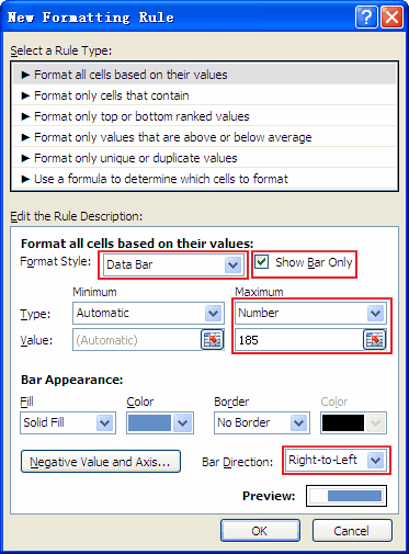
- In the New Formatting Rule window, under Format Style, choose Data Bar and click Show Bar Only. Under Maximum, Type: Number, Value: 185 (the max number of the two column). Under Bar Direction, choose Right-to-Left. See figure below.

- Click OK
Add Conditional Formatting for column C
- Select C2:C9.
- Under the Home menu tab, in the Styles group, click the Conditional Formatting button and choose New Rule....
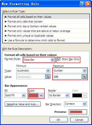
- In the New Formatting Rule window, under Format Style, choose Data Bar and click Show Bar Only. Under Maximum, Type: Number, Value: 185 (the max number of the two column). Under Bar Appearance, Color: Red Accent 2. See figure below.

- Click OK
Change the column width
The last step is change the each column width: Click Column A, press and hold CTRL, then click Column C, move mouse point to Column C header, drag the width to 150 pixels.
The final in-cell Tornado Chart result:
